Tutorial#
CLI#
GRouNdGAN comes with a command-line interface. This section outlines available commands and arguments.
To use the CLI, run the src/main.py script with the desired command and any applicable options.
Important
Use python3.9 instead of python if you’re running through docker or singularity.
$ python src/main.py --help
usage: GRouNdGAN [-h] --config CONFIG [--preprocess] [--create_grn] [--train] [--generate] [--evaluate] [--benchmark_grn] [--perturb]

GRouNdGAN is a gene regulatory network (GRN)-guided causal implicit generative model for
simulating single-cell RNA-seq data, in-silico perturbation experiments, and benchmarking GRN
inference methods. This programs also contains cWGAN and unofficial implementations of scGAN and
cscGAN (with projection conditioning)

required arguments:
--config CONFIG  Path to the configuration file

optional arguments:
--preprocess     Preprocess raw data for GAN training
--create_grn     Infer a GRN from preprocessed data using GRNBoost2 and appropriately format as causal graph
--train          Start or resume model training
--generate       Simulate single-cells RNA-seq data in-silico
--evaluate       Evaluate the data quality of the simulated dataset
--benchmark_grn  Evaluate the performance of a GRN inference method in inferring the ground truth GRN
--perturb        Perform a perturbation experiment using a trained GRouNdGAN model
There are essentially seven commands available: --preprocess, --create_grn, --train, --generate, --evaluate, benchmark_grn, and perturb. You must provide a configuration file containing inputs, parameters, and hyperparameters with each command through the --config flag.
Note
You can run commands individually:
python src/main.py --config configs/causal_gan.cfg --preprocess
Or chain them together to run all or multiple steps in one go:
python src/main.py --config configs/causal_gan.cfg --preprocess --create_grn --train --generate --evaluate
When chaining multiple commands, ensure that the supplied configuration file includes the required arguments for each command in the chain.
Config Files#
GRouNdGAN uses a configuration syntax similar to INI implemented by python’s configparser module.
We provide three sample config files in the configs/ directory:
causal_gan.cfg: for GRouNdGANconditional_gan.cfg: for cscGAN with projection conditioning (Marouf et al., 2020) and cWGAN.gan.cfg: for scGAN (Marouf et al., 2020) (we use this to train GRouNdGAN’s causal controller)
Most of the configuration file consists of hyperparameters. You mostly need to modify input and output parameters which we will go through in each section. GRouNdGAN isn’t very sensitive to hyperparameters. However, it is still advisable to test different choices of hyperparameters using a validation set.
Below is the demo causal_gan.cfg config file for training GRouNdGAN using the PBMC68k dataset:
[EXPERIMENT]
output directory = results/GRouNdGAN
device = cuda ; we will let the program choose what is available
checkpoint  ; set value to use a trained model

    [Preprocessing]
    10x = True
    raw = data/raw/PBMC/
    validation set size = 1000
    test set size = 1000
    annotations = data/raw/PBMC/barcodes_annotations.tsv
    min cells = 3 ; genes expressed in less than 3 cells are discarded
    min genes = 10 ; cells with less than 10 genes expressed are discarded
    library size = 20000 ; library size used for library-size normalization
    louvain res = 0.15 ; Louvain clustering resolution (higher resolution means finding more and smaller clusters)
    highly variable number = 1000 ; number of highly variable genes to identify

    [GRN Preparation]
    TFs = data/raw/Homo_sapiens_TF.csv
    k = 15 ; k is the number of top most important TFs per gene to include in the GRN
    Inferred GRN = data/processed/PBMC/inferred_grnboost2.csv

    ; "top" for selecting top k edges
    ; "pos ctr" for generating positive control GRNs (even indices 0, 2, 4... = top 1, 3, 5, ...)
    ; "neg ctr" for generating negative control GRNs (odd indices 1, 3, 5... = top 2, 4, 6, ...)
    ; note that k has to be a pair number for strategy=ctr
    strategy = top

    [Data]
    train = data/processed/PBMC/PBMC68k_train.h5ad
    validation = data/processed/PBMC/PBMC68k_validation.h5ad
    test = data/processed/PBMC/PBMC68k_test.h5ad
    number of genes = 1000

    ; this causal graph is a pickled nested dictionary
    ; nested dictionary keys are gene indices
    ; the dictionary is of this form:
    ; {381: {51, 65, 353, 664, 699},
    ; 16: {21, 65, 353, 605, 699},
    ; ...
    ; 565: {18, 51, 65, 552, 650}}
    ; In this example, 381, 16, and 565 are gene indices in the input dataset
    ; Each key's (gene's) value is the indiced of its regulating TFs in the input dataset
    ; A tutorial will be made available in the future.

    causal graph = data/processed/PBMC/causal_graph.pkl

    [Generation]
    number of cells to generate = 10000
    generation path ; will save to [Experiment]/output directory/simulated.h5ad if left undefined

    [Evaluation]
    simulated data path ; will use [Generation]/generation path if left undefined
    plot tsne = True # Note: has to be true in order to run miLISI
    compute euclidean distance = True
    compute cosine distance = True
    compute rf auroc = True
    compute MMD = True
    compute miLISI = True # plot tsne has to be True for this to work

    [GRN Benchmarking]
    grn to benchmark = path/to/inferred/grn.csv
    ground truth save path = data/generated/
    plots save path = notebooks/generated/
    compute precision at k = False
    k = 5
    compute pr = True

    [Perturbation]
    save dir = data/generated/

    ; tfs to perturb and perturbation values are paired. The two lists need to be of the same size.
    tfs to perturb ;= TF names separated by a space (ex: IRF8 CEBPA)
    perturbation values ;= Float values separated by a space to set respecive TF in tfs to perturb (ex: 0 100.2)

    [Model]
    type = causal GAN
    noise per gene = 1
    depth per gene = 3
    width per gene = 2
    critic layers = 1024 512 256
    labeler layers = 2000 2000 2000
    latent dim = 128 ; noise vector dimensions
    lambda = 10 ; regularization hyper-parameter for gradient penalty


    [Training]
    batch size = 1024
    critic iterations = 5 ; iterations to train the critic for each iteration of the generator
    maximum steps = 1000000
    labeler and antilabeler training intervals = 1

        [Optimizer]
        ; coefficients used for computing running averages of gradient and its square
        beta1 = 0.5
        beta2 = 0.9

        [Learning Rate]
        generator initial = 0.001
        generator final = 0.0001
        critic initial = 0.001
        critic final = 0.001
        labeler = 0.0001
        antilabeler = 0.0001


        [Logging]
        summary frequency = 10000
        plot frequency = 10000
        save frequency = 100000

    [CC Model]
    type = GAN ; Non-conditional single-cell RNA-seq GAN
    generator layers = 256 512 1024
    critic layers = 1024 512 256
    latent dim = 128 ; noise vector dimensions
    lambda = 10 ; regularization hyper-parameter for gradient penalty


    [CC Training]
    batch size = 128
    critic iterations = 5 ; iterations to train the critic for each iteration of the generator
    maximum steps = 200000

        [CC Optimizer]
        ; coefficients used for computing running averages of gradient and its square
        beta1 = 0.5
        beta2 = 0.9

        [CC Learning Rate]
        generator initial = 0.0001
        generator final = 0.00001
        critic initial = 0.0001
        critic final = 0.00001

        [CC Logging]
        summary frequency = 10000
        plot frequency = 10000
        save frequency = 100000
Project outline#
GRouNdGAN is structured as follows:
.
|-- .git
|-- .gitattributes
|-- .github
|   `-- workflows
|       |-- docker-build.yml
|       `-- documentation.yaml
|-- .gitignore
|-- .gitmodules
|-- Atkinson_Hyperlegible
|-- Beeline
|-- LICENSE
|-- README.md
|-- configs
|   |-- causal_gan.cfg
|   |-- conditional_gan.cfg
|   `-- gan.cfg
|-- data
|   |-- generated
|   |-- interim
|   |-- processed
|   |   |-- BoneMarrow
|   |   `-- PBMC
|   `-- raw
|       |-- BoneMarrow
|       |-- Homo_sapiens_TF.csv
|       |-- Mus_musculus_TF.csv
|       `-- PBMC
|-- docker
|   `-- Dockerfile
|-- docs
|-- notebooks
|-- requirements.txt
|-- requirements_computecanada.txt
|-- results
|-- scDesign2
|-- scGAN
|-- scripts
|   |-- monitor.sh
|   `-- train.sh
|-- sparsim
`-- src
Demo Datasets#
The provided docker image comes prepackaged with the unprocessed Mouse BoneMarrow (Paul et al., 2015) and Human PBMC68k (Zheng et al., 2017) datasets (data/raw/PBMC and data/raw/BoneMarrow) and human and mouse TFs, downloaded from AnimalTFDB (data/raw/Homo_sapiens_TF.csv and data/raw/Mus_musculus_TF.csv).
Note
If you have opted for a local installation, you can download these files from here and place them in data/raw/.
You can also do this in bash (you need curl and tar installed):
curl https://nextcloud.computecanada.ca/index.php/s/WqrCqkH5zjYYMw9/download --output demo_data.tar &&
tar -xvf demo_data.tar -C data/raw/ &&
mv data/raw/demo/* data/raw &&
rm demo_data.tar &&
rm -rf data/raw/demo/
Steps#
Preprocessing#
Attention
Don’t skip the preprocessing step, GRouNdGAN requires library-size normalized data as input.
To run our preprocessing pipeline, your config file should contain the following arguments:
[EXPERIMENT]

    [Preprocessing]
    ; set True if data is 10x (like PBMC)
    ; set False if you're providing an .h5ad file (like BoneMarrow.h5ad)
    10x = True

    ; If 10x = True, path to the directory containing matrix.mtx, genes.tsv, and barcodes.tsv
    ; If 10x = False, path to the .h5ad file containing the expression matrix
    raw = data/raw/PBMC/

    validation set size = 1000 ; size of the validation set to create
    test set size = 1000 ; size of the test set to create
    annotations = data/raw/PBMC/barcodes_annotations.tsv ; optional, leave empty if you don't have annotations
    min cells = 3 ; genes expressed in less than 3 cells are discarded
    min genes = 10 ; cells with less than 10 genes expressed are discarded
    library size = 20000 ; library size used for library-size normalization
    louvain res = 0.15 ; Louvain clustering resolution (higher resolution means finding more and smaller clusters)
    highly variable number = 1000 ; number of highly variable genes to identify

    [Data]
    train = data/processed/PBMC/PBMC68k_train.h5ad ; path to output the train set
    validation = data/processed/PBMC/PBMC68k_validation.h5ad ; path to output the validation set
    test = data/processed/PBMC/PBMC68k_test.h5ad ; path to output the test set
    number of genes = 1000
Then, run the following:
$ python src/main.py --config configs/causal_gan.cfg --preprocess
Once completed, you will see a success message. Train, validation, and test sets should be created in the paths defined under the [Data] section of the config file.
Expected output:
Successfully preprocessed and and saved dataset.
Train set: data/processed/PBMC/PBMC68k_train.h5ad
Validation set: data/processed/PBMC/PBMC68k_validation.h5ad
Test set: data/processed/PBMC/PBMC68k_test.h5ad
GRN Creation#
Note
GRN creation isn’t needed for scGAN, cscGAN, and cWGAN; you can skip the --create_grn command.
This command uses GRNBoost2 (Moerman et al., 2018) to infer a GRN on the preprocessed train set. It then converts it into the a format that GRouNdGAN accepts.
In addition to what was required in the previous step, you need to provide the following arguments:
[GRN Preparation]
TFs = data/raw/Homo_sapiens_TF.csv
k = 15 ; k is the number of top most important TFs per gene to include in the GRN
Inferred GRN = data/processed/PBMC/inferred_grnboost2.csv

; "top" for selecting top k edges
; "pos ctr" for generating positive control GRNs (even indices 0, 2, 4... = top 1, 3, 5, ...)
; "neg ctr" for generating negative control GRNs (odd indices 1, 3, 5... = top 2, 4, 6, ...)
; note that k has to be a pair number for strategy=ctr
strategy = top

[Data]
causal graph = data/processed/PBMC/causal_graph.pkl ; where to write the created GRN
By default, the top k most important regulating TFs of each gene will be included in the GRN (strategy = top). Alternatively, you can construct two separate GRNs, each containing half of these top k TFs per gene. By first setting strategy = neg ctr and then strategy = pos ctr, you generate two GRNs with identical densities and structural properties, based on the odd/even positions of the TFs in each gene’s ranked list. This strategy can be useful for controlled comparative analyses as both GRNs are equally sparse and are derived from the same underlying ranking.
Run using:
$ python src/main.py --config configs/causal_gan.cfg --create_grn
Once done, you will see success messages and the properties of the created GRN.
Expected output:
Using 63 TFs for GRN inference.
preparing dask client
parsing input
creating dask graph
4 partitions
computing dask graph
shutting down client and local cluster
finished
Successfully saved GRN inferred by GRNBoost2 GRN to data/processed/PBMC/inferred_grnboost2.csv

Causal Graph
-----------------  ------------
TFs                   63
Targets              937
Genes               1000
Possible Edges     59031
Imposed Edges      14055
GRN density Edges      0.238095
-----------------  ------------
Successfully saved GRouNdGAN causal graph to data/processed/PBMC/causal_graph.pkl
The causal graph will be written to the path specified by [Data]/causal graph in the config file.
Imposing Custom GRNs#
It is possible to instead impose your own GRN onto GRouNdGAN. If you’re opting for this option, skip the --create_grn command. Instead, create a python dictionary where keys are gene indices (int). For each key (gene index), the value is the set of indices set[int] coresponding to TFs that regulate the gene.

The GRN in the picture above can be written in dictionary form as:
causal_graph = {
    "G2": {"TF2", "TFn"},
    "G1": {"TF1"},
    "Gn": {"TF2", "TF1"},
    "G3": {"TFn", "TF1"}
}
Converting the key/value pairs into gene/TF indices, it becomes
causal_graph = {
    1: {4, 5},
    3: {0},
    6: {4, 0},
    2: {5, 0}
}
Then, pickle the dictionary:
import pickle

with open("path/to/write/causal_graph.pkl", "wb") as fp:
    pickle.dump(causal_graph, fp, protocol=pickle.HIGHEST_PROTOCOL)
Don’t forget to edit the causal graph path in the config file.
[Data]
causal graph = path/to/write/causal_graph.pkl
The GRN must be a directed bipartite graph
All genes and TFs in the dataset must appear in the dictionary either as key (target gene) or value (as part of the set of TFs)
Warning
Construct a biologically meaningful GRN!
Imposing a GRN with significantly different TF-gene relationships from those observable in the reference dataset will deteriorate the quality of simulated cells as generating realistic simulated datapoints and imposing the GRN will act as contradictory tasks
Training#
You can start training the model using the following command:
$ python src/main.py --config configs/causal_gan.cfg --train
Upon running the command above, three folders will be created inside the path provided in the config file ([EXPERIMENT]/output directory) and the config file will be copied over:
checkpoints/: Containing the.pthstate dictionary including model’s weights, biases, etc.TensorBoard/: Containing TensorBoard logs (saved as tfevent files)TSNE/: Containing t-SNE plots of real vs simulated cells
You can change the save, logging, and plotting frequency ([Training]/save frequency, [Training]/summary frequency, [Training]/plot frequency) in the config file.
Monitor training using TensorBoard:
tensorboard --logdir="{GAN OUTPUT DIR HERE}/TensorBoard" --host 0.0.0.0 --load_fast false &
We also provide two slurm submission scripts for training and monitoring in scripts/.
Expected output:
Done training causal controller step 0
Done training causal controller step 1
Done training causal controller step 2
...
Done training causal controller step 10000
Saved logs
Saved t-SNE plot
Done training causal controller step 10001
...
Done training causal controller step 200000
Saved logs
Saved t-SNE plot
Saved checkpoint
Done training GRouNdGAN step 0
Done training GRouNdGAN step 1
Done training GRouNdGAN step 2
...
Done training GRouNdGAN step 10000
Saved logs
Saved t-SNE plot
Done training GRouNdGAN step 10001
...
Done training GRouNdGAN step 100000
Saved logs
Saved t-SNE plot
Saved checkpoint
...
Done training GRouNdGAN step 1000000
Saved logs
Saved t-SNE plot
Saved checkpoint
Finished training
Note
Training time primarily depends on the number of genes and the density of the imposed GRN. It takes about five days with a very dense GRN (~20% density) containing 1000 genes on a single NVidia V100SXM2 (16G memory) GPU.
GRouNdGAN supports multi-GPU training, but we suggest sticking to a single GPU to avoid excess overhead.
GRouNdGAN trains for a million steps by default. It is not recommended to change this in the config file.
You can resume training from a checkpoint by setting
[EXPERIMENT]/checkpointin the config file to the.pthcheckpoint you wish to use.
In-silico Single-Cell Simulation#
One training is done, populate the [EXPERIMENT]/checkpoint field with the path of the .pth checkpoint you want to use in the config file (usually the latest).
[EXPERIMENT]
output directory = results/GRouNdGAN
device = cuda ; we will let the program choose what is available
checkpoint = results/GRouNdGAN/checkpoints/step_1000000.pth
You can change the number of cells to simulate in the config file (10000 by default)
[Generation]
number of cells to generate = 10000
generation path ; will save to [Experiment]/output directory/simulated.h5ad if left undefined
Then run
$ python src/main.py --config configs/causal_gan.cfg --generate
This will output a simulated.h5ad file to [EXPERIMENT]/output directory containing the simulated expression matrix.
Expected output:
Simulated cells saved to results/GRouNdGAN/simulated.h5ad
Evaluating Simulated Data Quality#
You can evaluate the quality of GRouNdGAN simulations using the following quantitative and qualitative metrics:
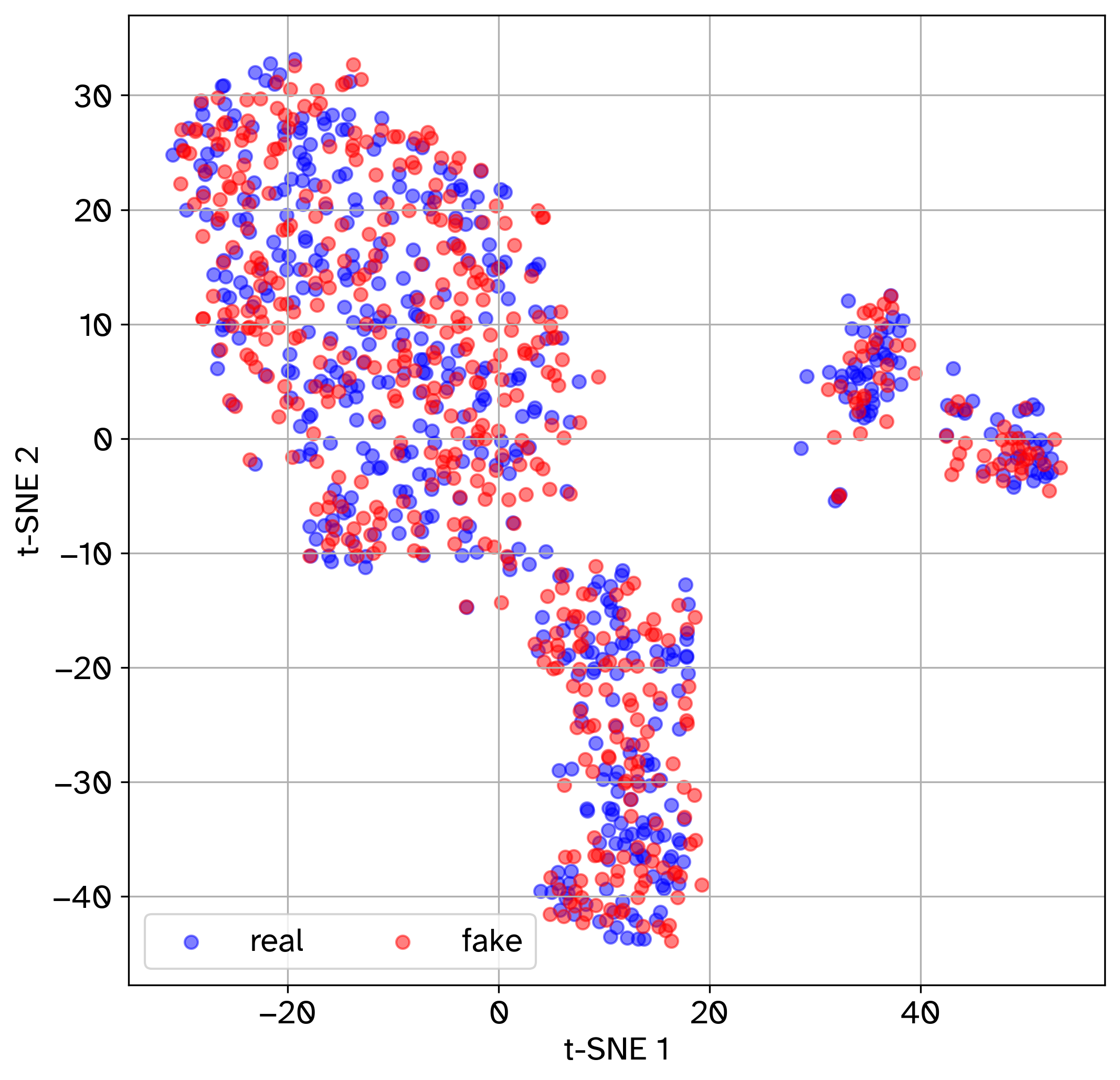
t-SNE plot of jointly embedded experimental and simulated cells.
Euclidean distance between the mean expression profiles of experimental and simulated cells.
Cosine distance between the mean expression profiles of experimental and simulated cells.
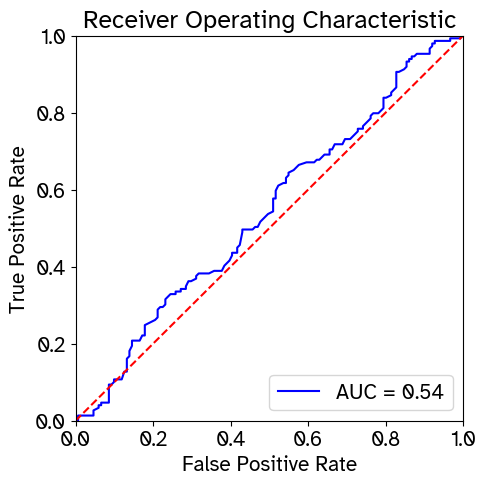
ROC curve and AUROC of Random Forest classifier distinguishing experimental from simulated cells.
Maximum Mean Discrepancy (MMD) for assessing distributional similarity between experimental and simulated cells.
Mean integration local inverse Simpson’s index (miLISI) of experimental and simulated cells.
The above metrics are computed between the test set and an equal number of cells sampled from the simulated data. In the t-SNE plot, greater overlap between experimental and simulated cells indicates better match. For the first three quantitative metrics (Euclidean distance, Cosine distance, and MMD), lower values reflect greater similarity. For the RF AUROC, values closer to 0.5 indicate that the classifier struggles to distinguish between simulated and experimental cells, which implies more realistic simulated data. For miLISI, values closer to 2 suggest better mixing of experimental and simulated cells. As a control, we also compute the Euclidean distance, Cosine distance, MMD, and miLISI metrics between two halves of the reference test set to serve as a point of comparison.
You can specify which evaluation metrics to compute by setting the appropriate flags in the configuration file.
[Evaluation]
simulated data path ; will use [Generation]/generation path if left undefined
plot tsne = True ; Note: has to be true in order to run miLISI
compute euclidean distance = True  ; or False
compute cosine distance = True
compute rf auroc = True
compute MMD = True
compute miLISI = True ; plot tsne has to be True for this to work
To run the evaluation with the specified configuration, use the following command:
$ python src/main.py --config configs/causal_gan.cfg --evaluate
Expected output:
t-SNE plot saved to results/GRouNdGAN/tSNE.png

Euclidean distance (real vs fake): 171.218017578125
Euclidean distance (control): 242.84738159179688

Cosine distance (real vs fake): 0.0003756880760192871
Cosine distance (control): 0.0007848143577575684

RF ROC plot saved to results/GRouNdGAN/RF.png
RF AUROC: 0.5410462687230544

MMD (real vs fake): 0.03008744777663175
MMD (control): 0.06244054076970418

miLISI (real vs fake): 1.89692891595357
miLISI (control): 1.8900128524031679
Benchmarking Inferred GRNs#
This command evaluates the reconstructed GRN (from GRouNdGAN-simulate data) against the ground truth GRN (used for simulation).
Configuration file arguments:
grn to benchmark = path/to/inferred/grn.csv
ground truth save path = data/generated/
plots save path = notebooks/generated/
compute precision at k = True
k = 15
compute pr = True
You will need to provide the path to the inferred GRN ([GRN Benchmarking]/grn to benchmark). The GRN has to be a tab-separated .csv file with three columns in this order:
TF
Gene
importance
Headers are optional — only column order matters.
Example inferred GRN csv:
Gata1       Hbb-bs  0.89
Tal1        Hbb-bs  0.74
Gata2       Gfi1b   0.52
If enabled via the configuration file, the benchmarking command will generate one or both of the following plots, saved to the directory specified in [GRN Benchmarking]/plots save path:
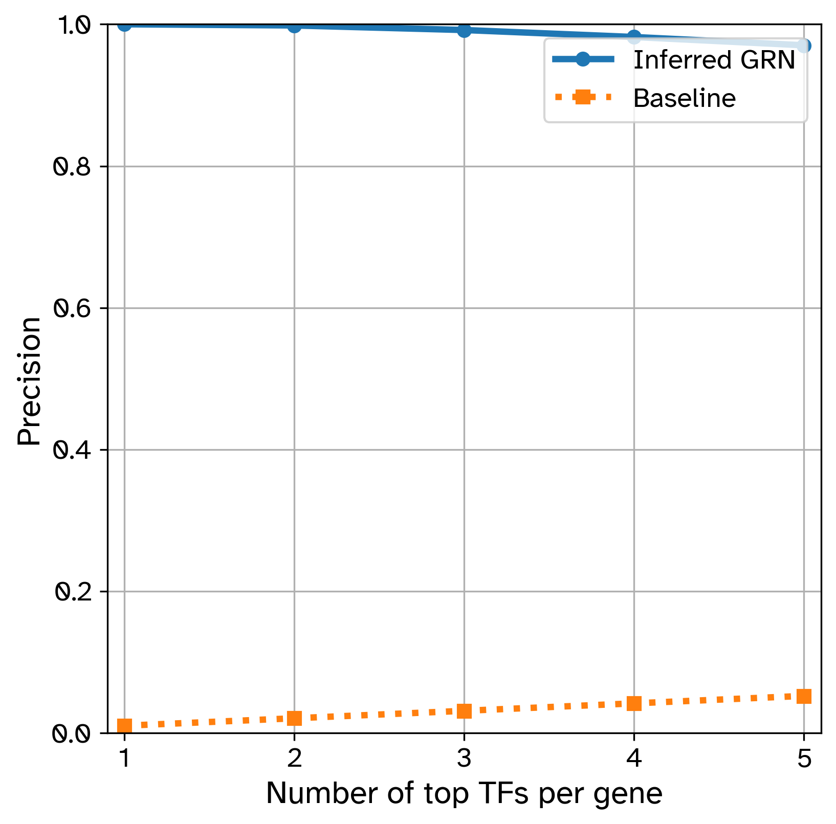
- Precision@k
If
[GRN Benchmarking]/compute precision at k = True, measures how many of the top-k (specified by[GRN Benchmarking]/k) inferred TFs for a gene are actually true regulators according to the ground truth.
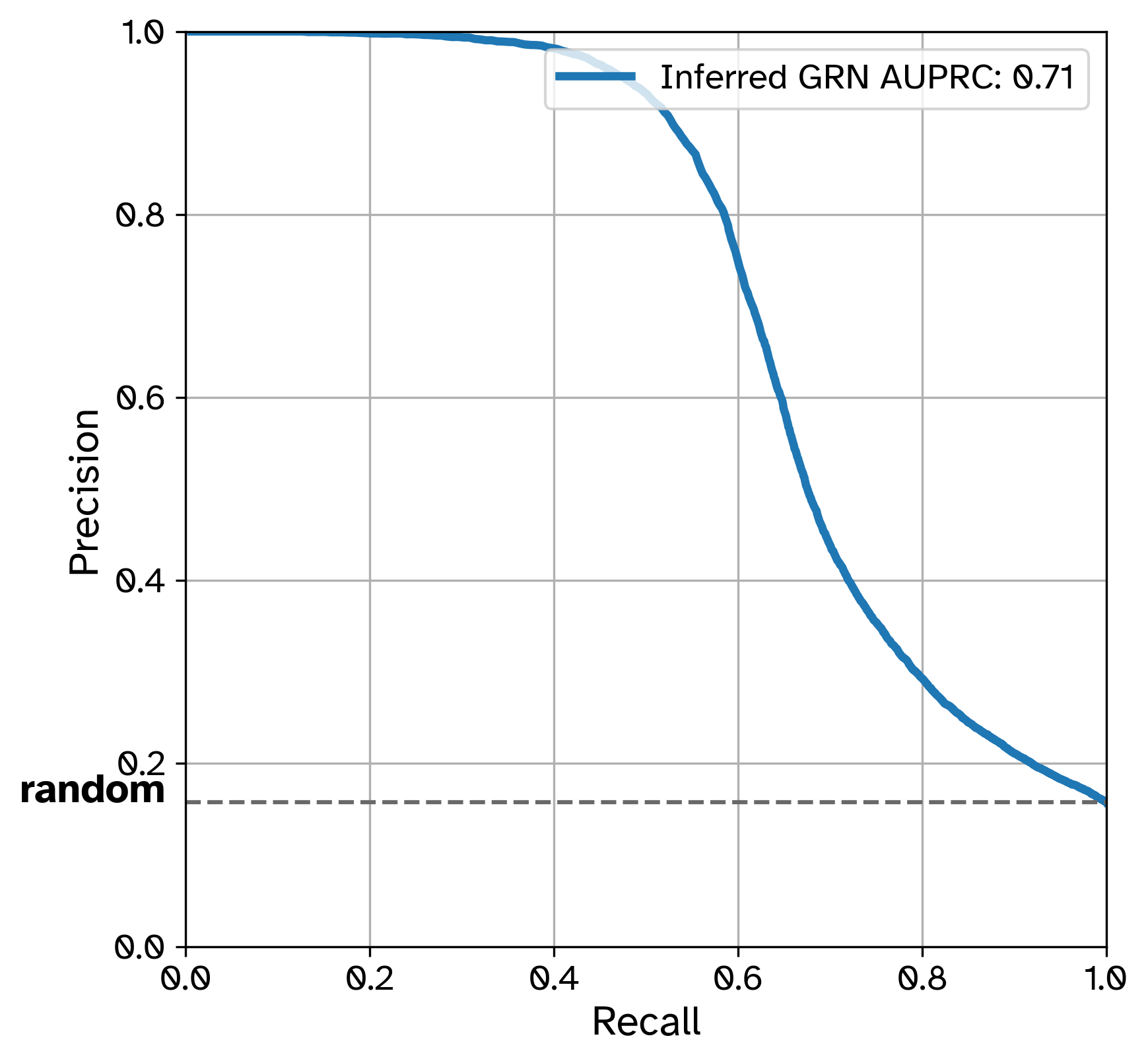
- Precision-Recall (PR) Curve
If
[GRN Benchmarking]/compute pr = True, a global Precision-Recall curve will be computed across all predicted edges in the GRN.
Both plots are saved as .png files, and any associated metrics (e.g., precision scores, AUPRC) are printed to the console.
Then run:
$ python src/main.py --config configs/causal_gan.cfg --benchmark_grn
Expected output:
Saved ground truth GRN to data/generated/ground truth GRN.csv

Inferred GRN precision at k: [1.0, 0.9983425414364641, 0.9918968692449356, 0.9820441988950276, 0.9703867403314917]
Baseline precision at k: [0.010526315789473684, 0.021052631578947368, 0.031578947368421054, 0.042105263157894736, 0.05263157894736842]
Saved precision at k plot at results/GRouNdGAN/Top_TF_precision.png

Inferred GRN AURPC: 0.71
Baseline AUPRC (random predictor): 0.15789473684210525
Saved PR curve at results/GRouNdGAN/PR_curve.png
Exporting Ground Truth GRN#
If you specify [GRN Benchmarking]/ground truth save path, the ground truth GRN will be exported as a CSV:
TF (regulator),Gene (target)
Gata1,Hbb-bs
Tal1,Hbb-bs
...
This can be useful for reference or external benchmarking tools.
Perturbation Studies#
Once trained, GRouNdGAN can sample from interventional distributions and perform in-silico TF perturbation experiments. These perturbations are applied to the same batch of cells, enabling matched case-control comparisons.
To run a perturbation, simply specify the list of TFs to perturb ([Perturbation]/tfs to perturb) and the corresponding values to which they should be set ([Perturbation]/perturbation values). The below configuration knocks out IRF8 and sets CEBPA to the value 100.2. The items in the list are separated by a space.
[Perturbation]
save dir = data/generated/

; tfs to perturb and perturbation values are paired. The two lists need to be of the same size.
tfs to perturb = IRF8 CEBPA ;= TF names separated by a space (ex: IRF8 CEBPA)
perturbation values = 0 100.2 ;= Float values separated by a space to set respecive TF in tfs to perturb (ex: 0 100.2)
Attention
Make sure perturbation targets ([Perturbation]/tfs to perturb) exist in the dataset and causal graph.
Once the configuration file is ready, run:
$ python src/main.py --config configs/causal_gan.cfg --perturb
Expected output:
Loaded GAN
Using checkpoint at results/GRouNdGAN/checkpoints/step_1000000.pth
Saved cells before and after perturbation to data/generated/
The cells before and after perturbation will be saved as after_perturbation.h5ad and before_perturbation.h5ad in the specified directory for secondary analysis.
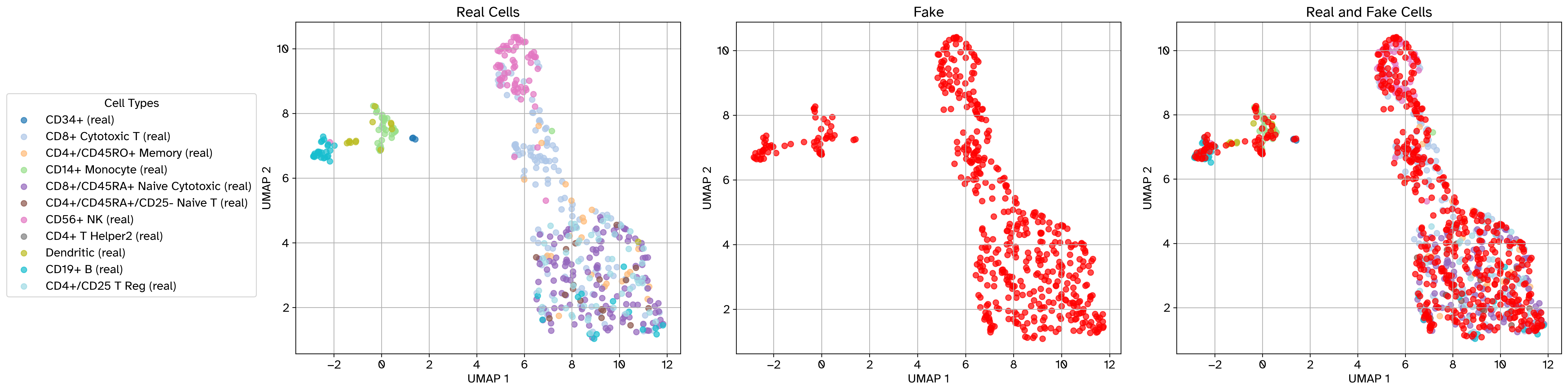
Example scatter plot before perturbation#
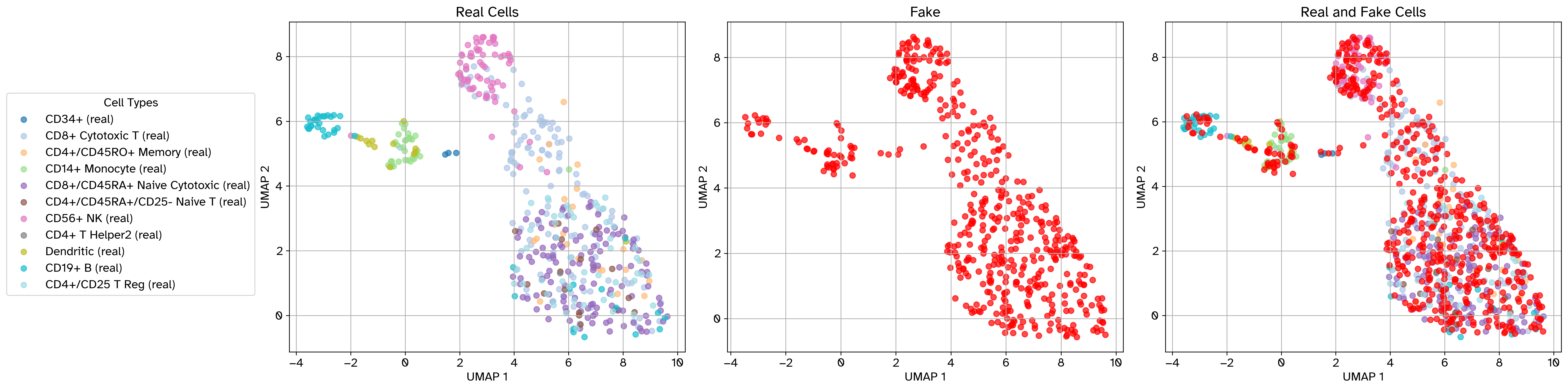
Example scatter plot after perturbation#
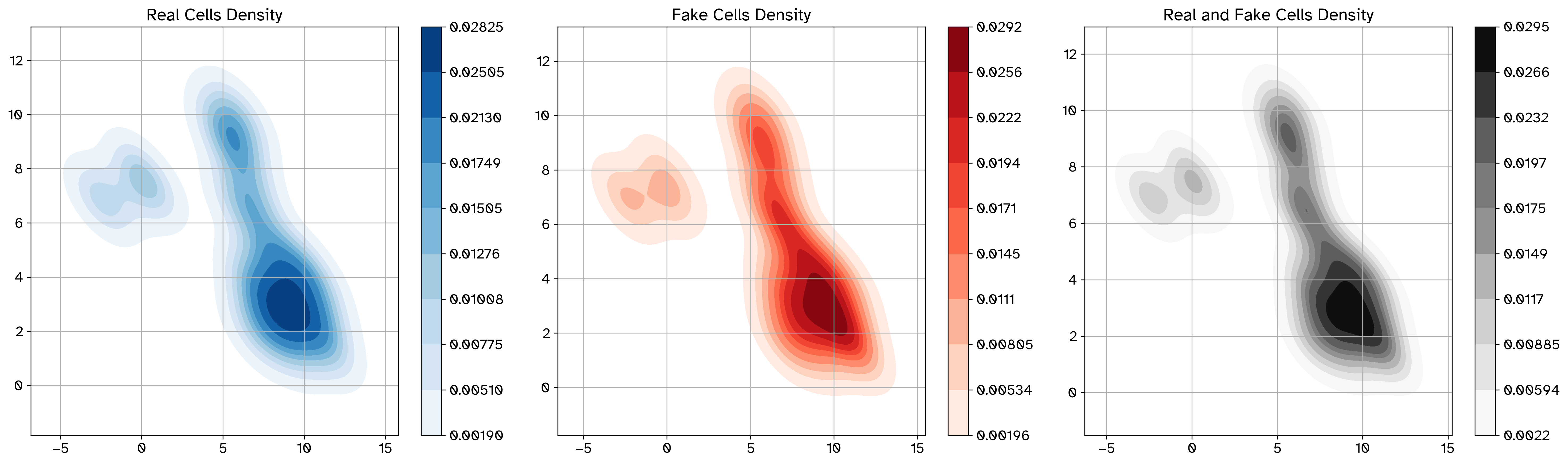
Example density plot before perturbation#
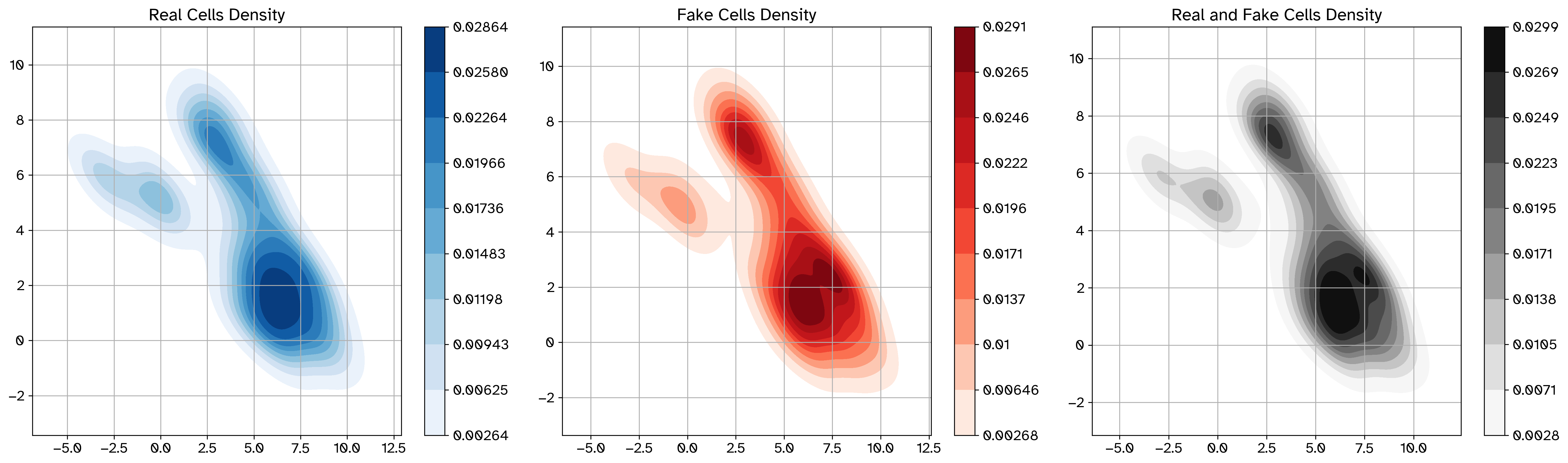
Example density plot after perturbation#
References#
Marouf, M., Machart, P., Bansal, V., Kilian, C., Magruder, D. S., Krebs, C., & Bonn, S. (2020). Realistic in silico generation and augmentation of single-cell RNA-seq data using generative adversarial networks. Nature Communications, 11(1). https://doi.org/10.1038/s41467-019-14018-z
Paul, F., Arkin, Y., Giladi, A., Jaitin, D. A., Kenigsberg, E., Keren-Shaul, H., Winter, D. R., Lara-Astiaso, D., Gury, M., Weiner, A., David, E., Cohen, N., Lauridsen, F. K. B., Haas, S., Schlitzer, A., Mildner, A., Ginhoux, F., Jung, S., Trumpp, A., … Tanay, A. (2015). Transcriptional heterogeneity and lineage commitment in myeloid progenitors. Cell, 163(7), 1663–1677. https://doi.org/10.1016/j.cell.2015.11.013
Zheng, G., Terry, J. M., Belgrader, P., Ryvkin, P., Bent, Z., Wilson, R. J., Ziraldo, S. B., Wheeler, T. D., McDermott, G. P., Zhu, J., Gregory, M., Shuga, J., Montesclaros, L., Underwood, J. G., Masquelier, D. A., Nishimura, S. Y., Schnall-Levin, M., Wyatt, P., Hindson, C. M., … Bielas, J. H. (2017). Massively parallel digital transcriptional profiling of single cells. Nature Communications, 8(1). https://doi.org/10.1038/ncomms14049
Moerman, T., Aibar, S., González-Blas, C. B., Simm, J., Moreau, Y., Aerts, J., & Aerts, S. (2018). GRNBoost2 and Arboreto: efficient and scalable inference of gene regulatory networks. Bioinformatics, 35(12), 2159–2161. https://doi.org/10.1093/bioinformatics/bty916